Russian Bridges, Eulerian Circuits, and Genome Assembly?

This is my attempt to better explain the intersection of math, bio, and computer science. Most strict examples used for understanding in the article are in Pavel Pevzner and Phillip Compeau’s books, but formatted and expanded upon by me.

The intersection of mathematics and biology is really something beautiful to think about. Of course it makes sense that our DNA follows the same underlying principles as literally everything else in the world (math), but the dots connect in such a way that it makes everything really clear.

As I continue on my journey to one day work at the intersection of biology and engineering, ideas like this are almost central to my understanding and also appreciation of biology and why I love it in the first place.

A very important example of this is the unique crossover of graph theory with a critical process that is the precursor to every major discovery in biology: genome assembly.

My objective with this article is to help you not only learn more about computational biology, but also explain why I think everyone should be going crazy about computational biology and the potential it has with a simple, clear example.

Okay, I talked a lot about the poetry of math and science, but what about the technicalities? Why is understanding graph theory and recreating our genome so important?

It all starts with understanding the human genome in its entirety.

I’ll let David Gifford at MIT explain why genome assembly is fascinating because he sums it up pretty well.

“(Genome assembly) is at the bedrock of all modern biology. We rely upon genome references for almost everything in terms of studying evolution, looking at the structure of genes… it’s really a very fundamental concept”.

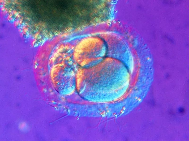
What genome assembly refers to is the process of organizing subcomponents of DNA to get a representation of genetic information that can describe the entire organism.

The human genome for example is just a catalogue of every single DNA sequence that our body’s use. Think of it as the dictionary of the human species. If you’ve taken a high school biology class, you’ll know that humans have 23 pairs of chromosomes (chromosomes are a much more condensed version of several DNA molecules).

Each chromosome of course is made up of a histone backbone that binds to these DNA molecules, and when we sequence each and every unique DNA sequence in each genome, we get a very long dictionary of sequences, almost three billion base pairs long DNA.

The skeptical scientist or engineer might look at this and say “3 billion base pairs is long. How on earth can we even read this much data at once?”

Well, you’re not wrong. Sequencing 3 billion base pairs is not only difficult computationally speaking, but our technology is still unable to sequence a genome in 1 go, primarily because of the information loss that comes from extracting a super long sequence.

If you can recall the Human Genome Project the race to map the entire human genome was very difficult for this exact reason.

Production challenges in the lab such as getting enough samples, preventing contamination, getting accurate representations of an actual sequence and mapping its function are all some of the primary hurdles that we’re slowly getting over (we technically just sequenced the entire genome this year).

These are all fundamental problems a part of genome assembly. To sequence or read your genome, you first need to find a way to get smaller representations of your genome and then put them together to initiate sequencing.

Now, we were able to sequence the “human genome” yes, but what about the billions of people on Earth and other organisms whose genomes we could sequence? How much more could we learn about ourselves and the world around us if we could find better and more accurate ways to assemble our genome?

That’s the premise. To first sequence and interpret your genome, you first need to be able to assemble it.

How do we most effectively assemble the genome of an organism?

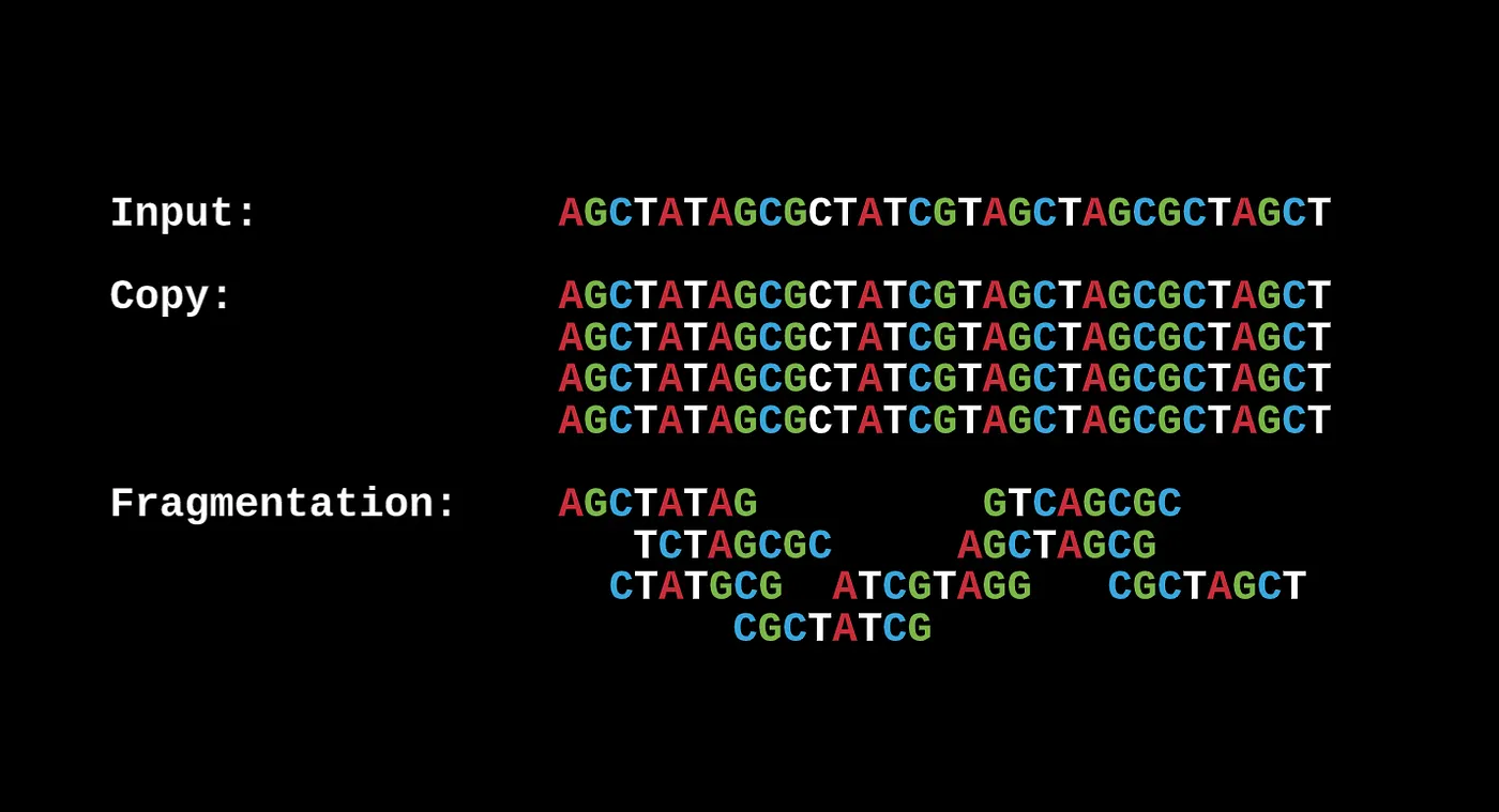
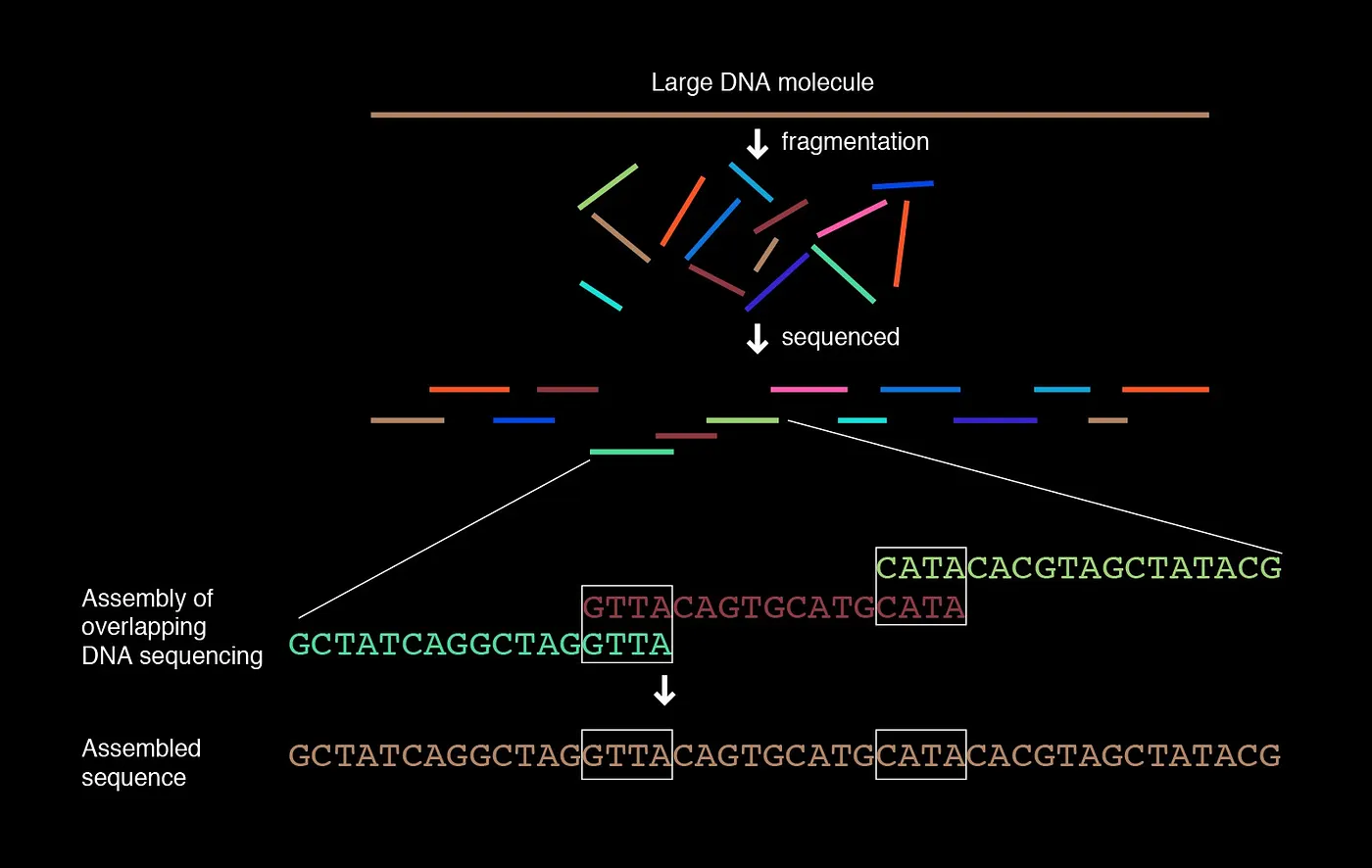
The basic principle is that we want to collect a set of fragments from several DNA copies or contigs that contain central but unconnected bits of information and then combine them to find the correct order of these fragments.

Contigs or contiguous sequences are combined through scaffolds which identify areas of overlap between specific contigs. We can overlap certain contigs together in the form of read pairs. This can be considered the prefixes and suffixes of a word, and we can use them to arrange the words in order for our dictionary given our current scaffold or category by letter.

Another way to think about this is that we have some gaps in our sequence because we may have lost a few reads initially.

If you know what the last part and first part of these contigs are, you can bridge them with a contig that contains both of these at their respective start and ends.

There’s a lot of different pipelines you can use after this for arranging and ordering these scaffolds such as sequence tag sites which can help order certain scaffolds in the actual chromosome. Ultimately, these can be inferred and interpreted to produce the final genome map or the dictionary in our analogy.

While this process, known as de novo whole-genome shotgun assembly, seems simple, it’s anything but. Problems such as mutations or unordered reads from initial amplification or denaturing all complicate this process, let alone make it difficult for us to find the exact order that these contigs should be arranged in.

Some problems and key barriers are, but not limited to:

1. Since DNA is double-stranded, there is no way of knowing which strand a given read derives from, meaning that we don’t know whether to use the read or its reverse complement for a given reconstruction for a specific direction (3’ or 5’).
2. Reading a genome from left to right is not very useful as the level of complexity for most algorithms increases as you introduce new nucleotides to the sequence. Not only are you not necessarily sure of what fragments, patterns, or statistical anomalies you’re looking for, but it becomes harder to reduce this scope with an increasing length.
3. Modern sequencing machines often have errors that make it difficult to specifically “read” a genome in its entirety. → Sequencing errors complicate genome assembly because they can often prevent us from identifying overlapping reads
4. Some regions of the genome may not be covered by any reads because of a lack of knowledge, making it impossible to reconstruct an entire genome. These are often blindspots in our own understanding where computational sequencing methods and genome maps can help prevent.

This is known as de novo assembly where we need to assemble a set of reads from scratch with no prior knowledge or reference.

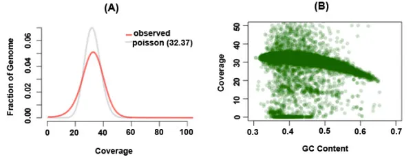
A quick detour: S/O to MIT Open Courseware: we can design an algorithm specific to the genome based on the coverage we have. Coverage is another name for how many nucleotides we have in total across all reads and what percentage they make for the entire genome length.

We can use a poisson distribution to model the probability that a base is covered in our reads or not since the data we have is essentially random and independent. The coverage can be considered the µ or mean of the distribution, and thus the variance is also equal to the coverage in this case. Note that coverage is relative to the whole genome.

As a result, if we were to try and find the probability that a base is not covered, it would make up the part of the graph up to the mean or µ (thus the factorial of x!) because we’re trying to find the sum of each probability.

Why is this useful? Well, you can use the probability to find key overlap points, especially repeats in your reads, but I’m getting ahead of myself.

Back to normal: TLDR: DNA assembly is important, challenging, but also quite fun to tackle. I’ve only really talked about DNA assembly, but how do we frame this into a computation problem?

Framing the problem from randomized strings to approaches.

There’s a few things we need to recognize in our problem right off the bat. For one, we can assume that the coverage is nearly almost perfect (which is really unrealistic) but does help for building intuition early on. We also know that most of these reads are the same length, so that can easily help us recognize overlaps.

Given what we know about the initial approach to assembling said genome, it’s pretty obvious that we can assemble these configs by observing their overlapping areas (prefix and suffix) to establish order.

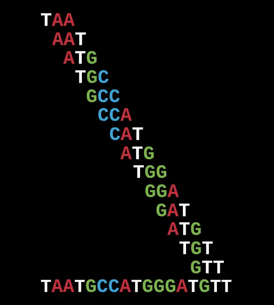
The same system can be used to find the first and last k-mer in the arrangement based on whether their prefix or suffix overlaps with any other k-mer in the set. In our case, this is TA in TAA and TT in GTT.

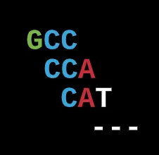
The reads can be arranged in order based on their overlap as follows.

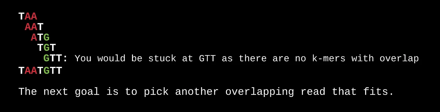
Based on the sequence and set of steps above, it’s pretty clear that this approach isn’t all that useful for finding a finalized output since we can get stuck at local minimums (low-depth sequencing). Even still, it is possible to get to a final output after several random iterations.

But as I said above, this could work well for smaller sets of reads based on trial and error but even still it can become problematic because of repeating k-mers or overlap areas.

While some overlap areas can be much more common in a given set of reads, others are less likely to and thus you can have several potential options and paths that may lead you down the incorrect arrangement (note, this doesn’t even account for the potential mutations and errors).

It’s almost impossible to effectively calculate the probability of an overlap because the probability solely depends on the kind of overlap and the overall set of reads.

Take the sequence ATTTATATTTTATAT and the 2 reads TT and AT. The probability of TTA occurring in the sequence is 5/14 which is equal to AT, but in reality, TT would have a much higher probability than AT since TT can overlap with itself. Again, this is a simplified example, but repeats do make it more difficult to find correct overlaps.

Based on this simplified example, I’ve made it pretty clear that random iterations and guess-check is a pretty inefficient idea. This is where representations of our data can become really useful for not only removing redundant reads but also finding quick and easy paths that are objectively correct.

A quick intro on graph theory, cycles, and notation.

For starters, know that a graph is really just a fancy way to visualize connections between data. The data being nodes in the graph and the connections being the edges.

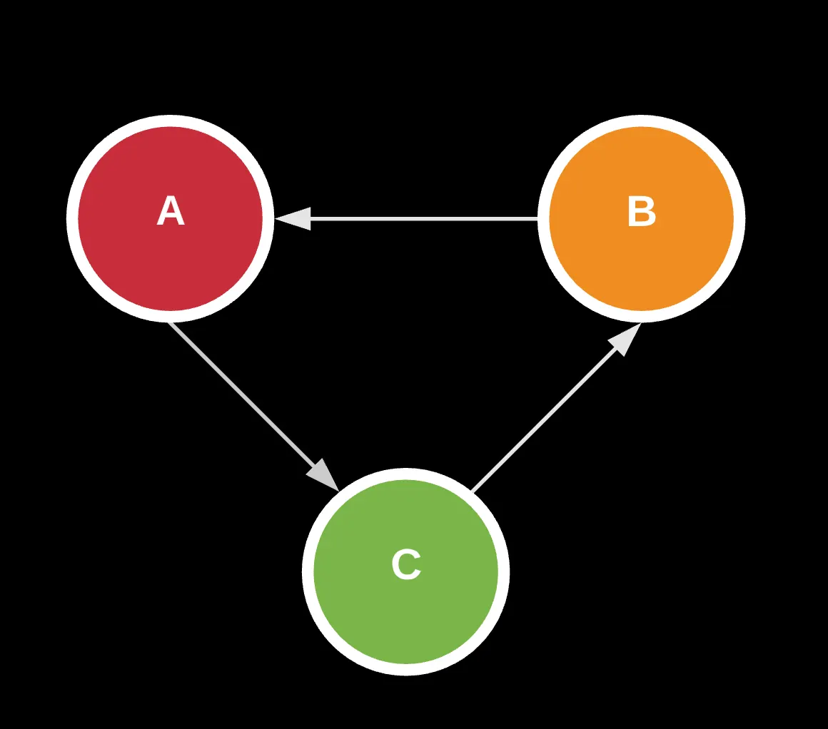
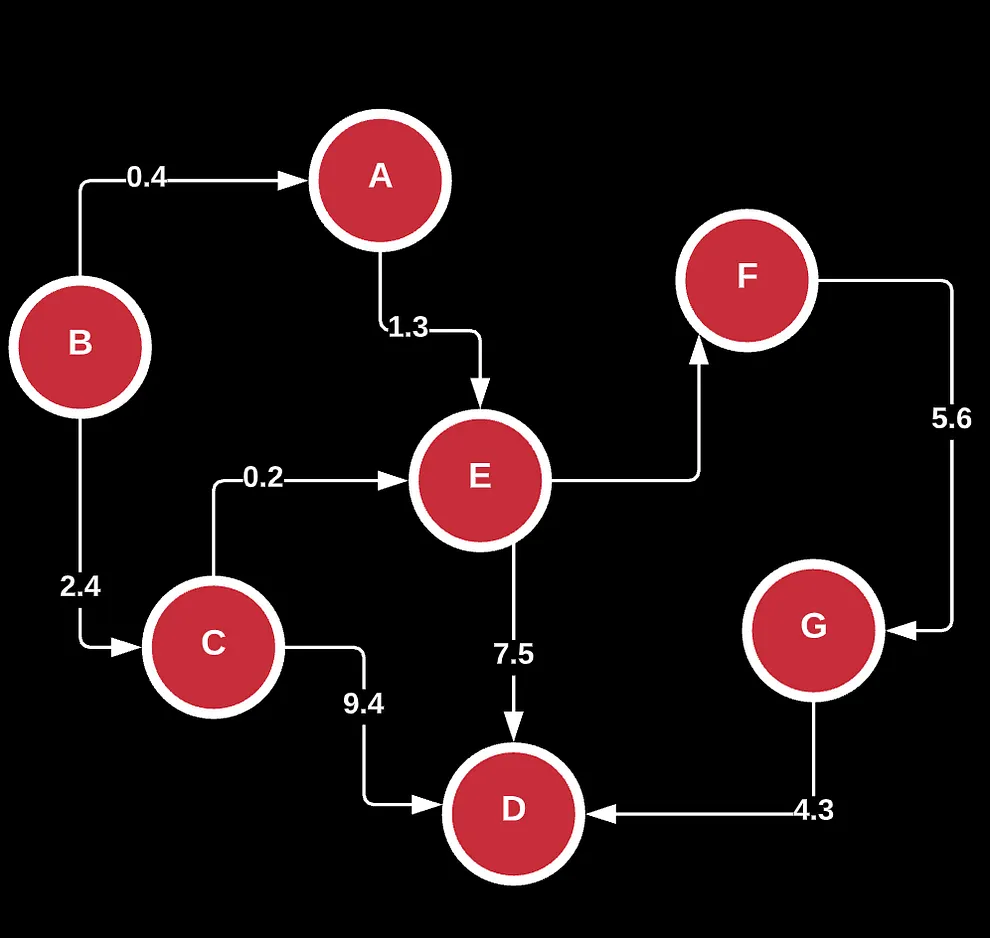
Take the following for example. This is known as a directed graph which showcases one-one or one-many relationships.

Here, we see a set of nodes labeled V and a set of edges or relationships labeled E. Using this, we can draw connections to describe how these adjacent pairs connect with each other.

Now, let’s say I wanted you to find all possible combinations of a, b, c as a string, starting with the letter a. With this visualization, it’s pretty obvious that you can create 2 representations by taking 2 different walks on the graph: (a -> b -> c) and (a -> c -> b). Note that because the graph is directed, we can’t do (a->b->a) or anything like that.

In our case, this is really good for finding orders and arrangements, and thus reduces the complexity of our graphs by a large amount. This provides constraints to our problem and can be phrased and solved using graph theory.

There’s also other graphs such as weighted directed acyclic graphs (neural nets), undirected, trees and arborescence parts of rooted trees, bipartite, and more.

If you’ve noticed already, graphs are typically distinguished by direction, the nature of their edges/connections (u and v), and the number of cycles.

With our visualization, there are a lot of problems that encompass graph theory from the shortest-path problem (your GPS routes), measuring connectivity and balance (whether all nodes are connected to each other in some way with certain restraints), and finding self-contained, strongly connected components.

Directed graphs and string graph overlap layout consensus

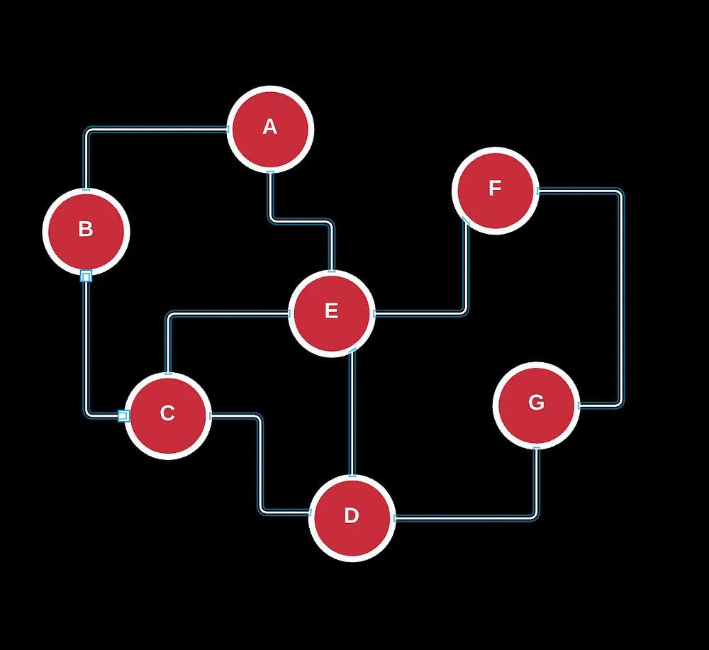
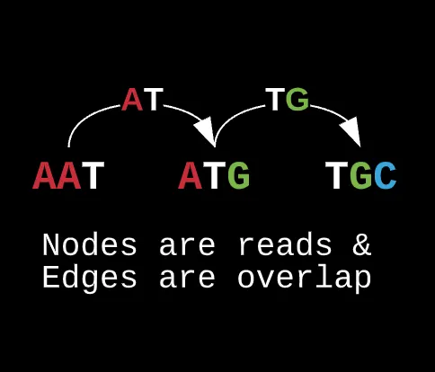
To make an easier representation of our reads and overlaps, we can go back to our prefixes and suffixes for notations. Assuming some prefixes connect to other suffixes and there are several repeats, we can construct a graph, specifically a directed graph whose nodes represent the actual reads and edges represent the prefix or suffix.

This approach is formally called the Overlap–layout–consensus approach where each read is mapped to every other read in the sequence in the graph, and overlaps are determined by the edges.

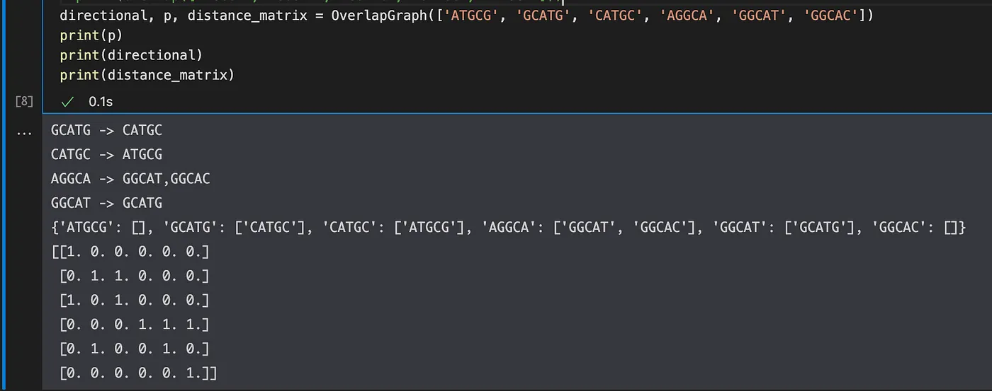
Notice that this is a balanced, strongly-connected graph where through some path, each node or config is connected to the other. I also generated some code samples below to help you process and experiment with this

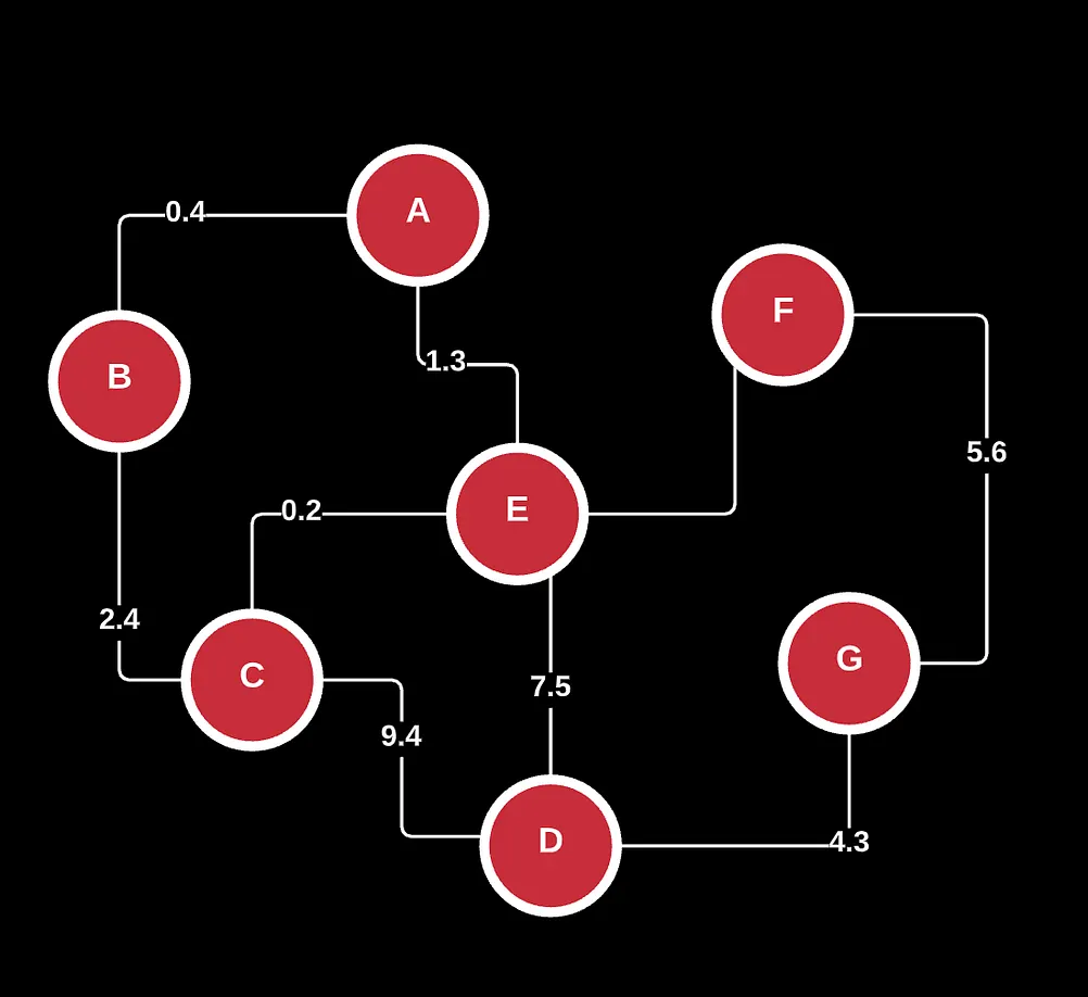
The following are dictionary and distance matrix representations of our graphs. What you’re really solving here for given the fact that each read is of the same length and same goes for the overlaps, you are essentially trying to find the shortest string sequence from a set of reads by maximizing how much each read can overlap with another (increasing coverage -> 1).

Given this graph, how can we actually find the correct order and direction for our final assembled genome?

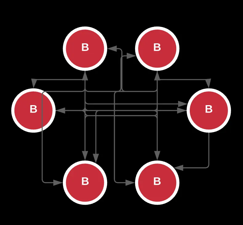
If we look at it from a graph, we know that the optimal solution can be found by visiting each node or read once only, and the only way to get there is to find the ideal order of reads we should visit. This is a lot more difficult than it seems because most graphs can be cyclic or have self-contained components because of repeats in our overlaps.

This kind of walk is known as a Hamiltonian Path**.**

A hamiltonian path is a special kind of walk of the graph where each node in the graph is visited exactly once, regardless of how it gets there. If during our walk, we end up at the same node we started at, this is known as an hamiltonian circuit.

Again, this seems easy to solve but the truth is that this problem is considered NP-complete. Why? Well because the only way to solve for the hamiltonian circuit is the brute force method we had initially tried.

You can see the proof for this here from CSC 463: http://www.cs.toronto.edu/~ashe/ham-path-notes.pdf

I kind of lied in the sense that our graph representation for this specific instance. The brute-force algorithm is considered to have a time complexity of O(N²). While the brute force algorithm works to minimize the total cost along the path or simply put, find the shortest common superstring that is made up of all the reads, this doesn’t work for hundreds of millions of reads.

So what do we do now? Let’s reframe the question a little.

I think a CS major would probably not choose to go use a Greedy String algorithm, and this is good because of the repetition of reads in a typical genome.

We could try to maximize overlap as a result, and so you would get stuck when 2 repeats are set together. This is getting confusing. Let’s break it down a little more.

We know that the properties of our graph representation for our contigs needs to be in such a way where a path must be able to connect all possible contigs without repeats.

Another point we want to add is that we want a simplified representation of the graph, or the graph should be untangled.

In this instance, we can’t represent the k-mers as nodes because the directed edges only represent the suffix overlap with the next node’s prefix. Rather, if we want to maximize overlap and coverage, you would want the actual prefix and suffixes as the nodes in the graph whereas the k-mers act as the edges or glue that connect each node together.

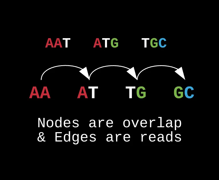
For real world data, most of the contigs collected will have repeats from multiple copies, they can have potential mutations, or missing reads for that matter. If we were to use a hamiltonian to draw out a path and sequence, it limits the ability for reconstructing a genome later on with specific hyperparameters such as error thresholds (known as hamming distance) or eliminating repeats (which we’ll get into later).

Note how this representation can change if we decide to alter the actual length of our prefixes and suffixes while preserving the edge’s contents as the actual reads.

What this also allows us to do is reduce the total edges in the graph as for a traditional hamiltonian, there could have been several connections from one node to another whereas here, each prefix is connected to a specific suffix only by the read resulting from their overlap and nothing else.

For example, if we had repeating reads such as ATG from the above example, a hamiltonian would have had to given those reads single nodes since for the hamiltonian path to work, each node would have to be visited once. As a result, you can’t overlap any nodes to simplify the graph.

This is clearly outlined in the formal definition of an overlap graph with a hamiltonian walk:

A graph is an overlap if its vertices may be put into a one-to-one correspondence with intervals on a line, such that two vertices are adjacent iff there intervals partially overlap, that is, they have non-empty intersection, but neither contains the other.

In this new graph, since our new representation stores the reads as the edges in our graphs instead of the nodes, we can now define our new criteria for a path as any walk that goes through each edge in the graph exactly once.

Our cycle would then be simply the same thing but ending at the node we started on.

This graph is known as a De Bruijn graph and it’s quite useful.

De Bruijn graphs are also directed graphs, but have the property of being Eulerian. What does this mean now?

Well, have you heard of the seven bridges of Konigsberg?

The city of Konigsberg has seven bridges that allow its visiters to cross the different parts of the Pregel river.

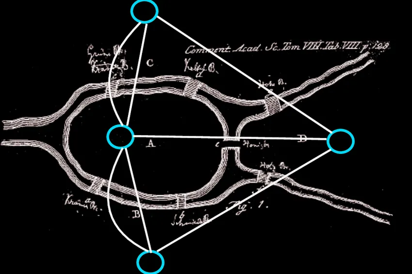
The city wanted to find a path such that a visitor can start at any bridge and return to that same bridge by crossing every bridge in the city. Essentially, this was known as our Hamiltonian path for this graph but it was impossible to do so.

That’s because for a Hamiltonian path to be true, each node must have an even degree whereas here, each node has an odd degree.

What came out of it however was Leonhard Euler’s proposed solution that satisfied a part of the constraint. He showed that the graph had a Eulerian path where each visitor had the ability to cross every bridge exactly once, but never come back to where they had started.

So let’s introduce the idea of a Eulerian graph, path, and everything in between.

A graph can be Eulerian if there is a path (Eulerian path) that visits each edge in the graph exactly once. Not every graph has an Eulerian path however, and not each graph with an Eulerian path has an Eulerian cycle.

These properties are somewhat useful for genome assembly, but let’s address identifying some properties of a Eulerian graph. A directed graph can only be Eulerian if every vertex has an equal degree apart from 2 of the vertices where 1 has an in-out degree of 1 and the other has an out-in degree of 1 as well.

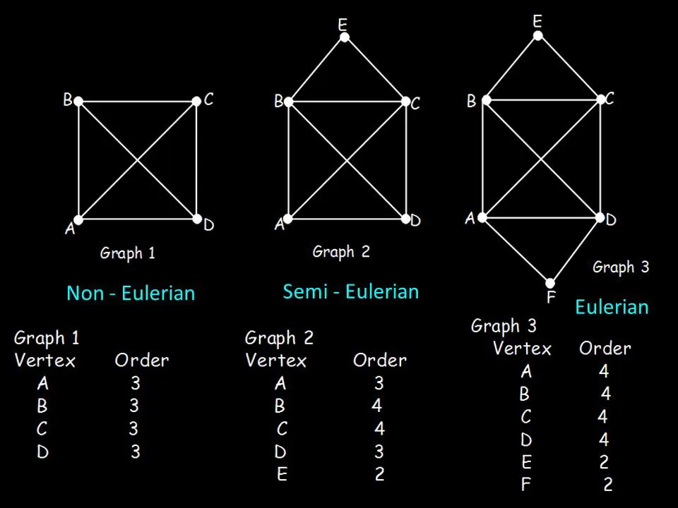
Why is this important? Well, let’s define what degree means first. The degree of a node is determined by the difference between the number of edges that connect to said node and the edges that the node has connected to other nodes.

Well, in order for us to be able to start a Eulerian path, the starting vertex needs to only have one way back to the node since that would allow the path to end.

In this case, B is the starting node since it only has 1 incoming edge and 2 outgoing edges. Therefore, node B has an o(B) of 2 and an i(B) of 1. The degree of this is |o(B) — i(B)| = 1. In a similar fashion, C is the end node because it has 2 incoming edges and 1 outgoing edges. Therefore, node C has an o(C) of 1 and an i(C) of 2.

All other nodes have an even degree where the difference between their o(v) and i(v) is always an even number, regardless of what the i(v) and o(v) are.

So going back to our De Bruijn graph, the starting prefix will always be the node in the graph that only has 1 outgoing edge if the genome is linear, and a degree of 1 if the genome is circular.

Our Eulerian path is useful for a few reasons, primarily the fact that it helps prevent the loss of sequences and repeats in our data.

For Hamiltonian graphs, some walks can visit each node but fail to take in all possible repeats in the correct order. Additionally, solving for a Hamiltonian path becomes exponentially more difficult as the genome increases in length.

We have now reframed our problem to be a Eulerian path finding problem. In order to find that said path however, we need to be able to construct a said De Bruijn graph that can help out visualize the path.

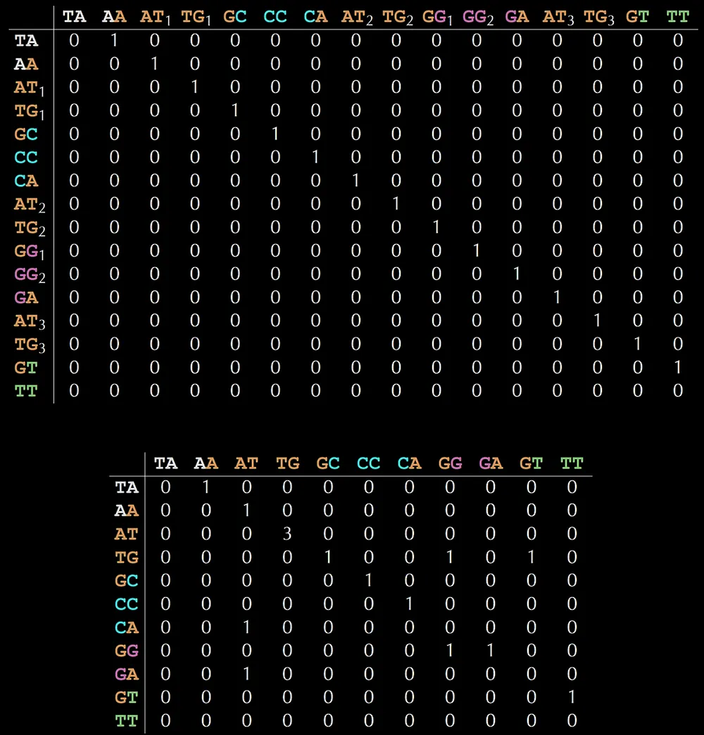
Given a set of contigs, you can construct a De Bruijn graph using a simple script:

The output of this represents the De Bruijn graph in a dictionary format.

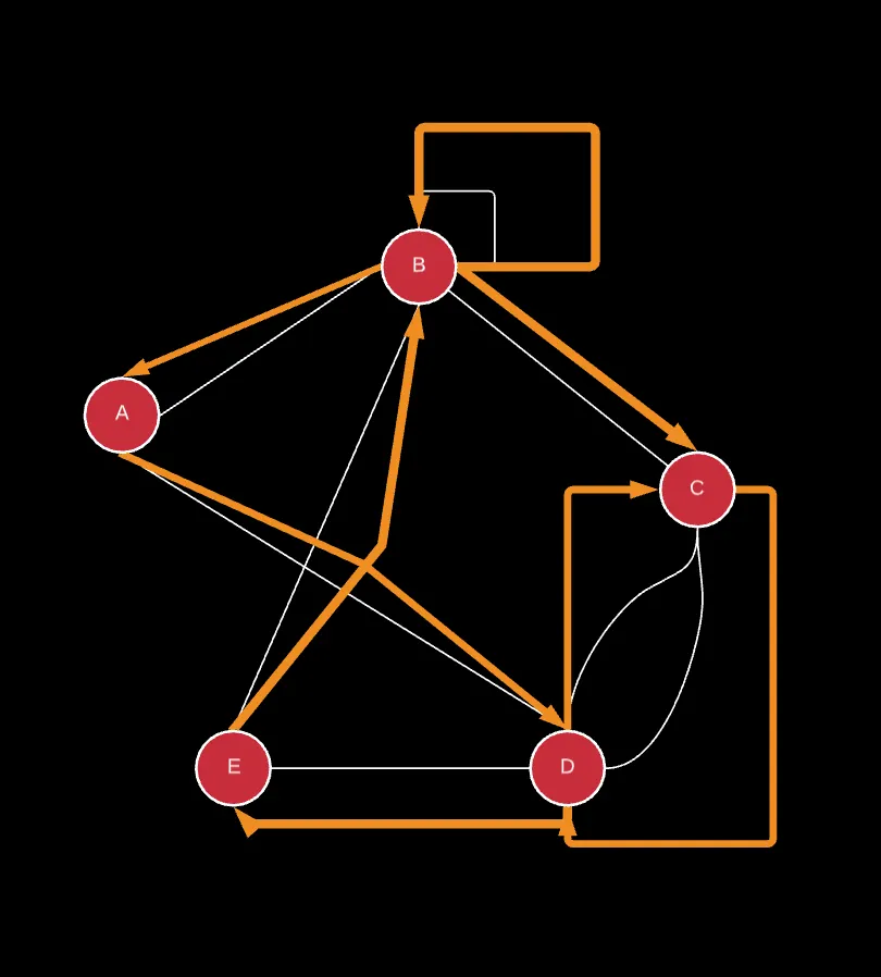
Now comes the hard part which is finding a Eulerian path in our De Bruijn graph. If you were to create a brute force method that checks whether each edge was used once or not would be ineffective for a larger graph, primarily because you can get stuck at many local Eulerian cycles at a given walk.

We can use this to our advantage, where instead of creating several random walks, you can randomly walk through the graph until you reach a stop point. This could be when you end at the same node that you started off at or if there are no other edges to walk on.

This can help identify the end of a graph quickly once you hit a dead end, and then backtrack to cross each and every edge of the graph.

A popular way to demonstrate this is by breaking up the graph into several one-directional graphs where each node has an o(v) and i(v) of 1. This is similar to a random walk of the graph, and if the graph is truly Eulerian, then each node apart from 2 will have an unused edge.

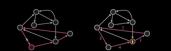
Once you reach the end of a cycle or path, you can backtrack until you read a node with an unused edge. That can now become the starting point for your next walk and you can eliminate the edges you’ve visited in the previous walk.

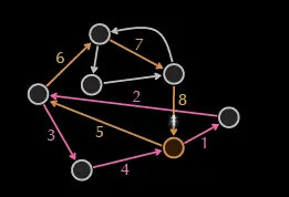
This next cycle ends at another node with an unused edge, and this process continues until all edges are traversed. This algorithm works well for a cycle since the graph is balanced, and a similar process works for a Eulerian path where the only constraint is that the last node of the network will be determined in the first walk since that graph will always be nearly unbalanced.

This is known as the Hierholzer’s algorithm, and is explained well by this great video tutorial which you should watch to gain some intuition.

This is a simple script that implements the Eulerian cycle walk:

Using this example dataset, you can then check the answer for your Eulerian cycle here.

For a Eulerian path, we can implement a similar algorithm for a De Bruijn graph (just like the Eulerian cycle) as seen below.

Using this example dataset, you can use the following formatting function to validate your answer.

We’ve worked on some of the more fundamental parts of Genome Assembly, but now we need to work on the practical parts.

One thing that bugged me initially when learning about genome assembly was whether the smaller parts of our solution, such as the assumption that overlaps are k-1 in length or there is only one possible solution, discredited a lot of what I was doing.

Well, not so much. The purpose of this process is to better learn how genome assembly is done with real world data, and having ideal examples only strengthens our foundation.

With that being said, let’s jump into reads, specifically their lengths. One key point to note is that the longer the read length, the more accurate the final sequence will be.

Longer reads have the advantage of having larger overlap coverage, thus making it more stricter for overlaps compared to shorter sequences where the overlap length has limited room for error.

This also helps with finding mutations or errors early on in the pipeline and removing amplification bias where some parts of the genome have a greater number of copies than others (as seen with the comparison above).

As of now, most recommended read lengths (k) are approximately 300 nucleotides long. This makes sense since the longer the read lengths become, the less tangled our graphs become and the closer you get to having the original genome from the start.

For 3 billion long genomes however, 300-mer contigs are almost nothing. This not only presents several issues in accuracy but also makes computation harder.

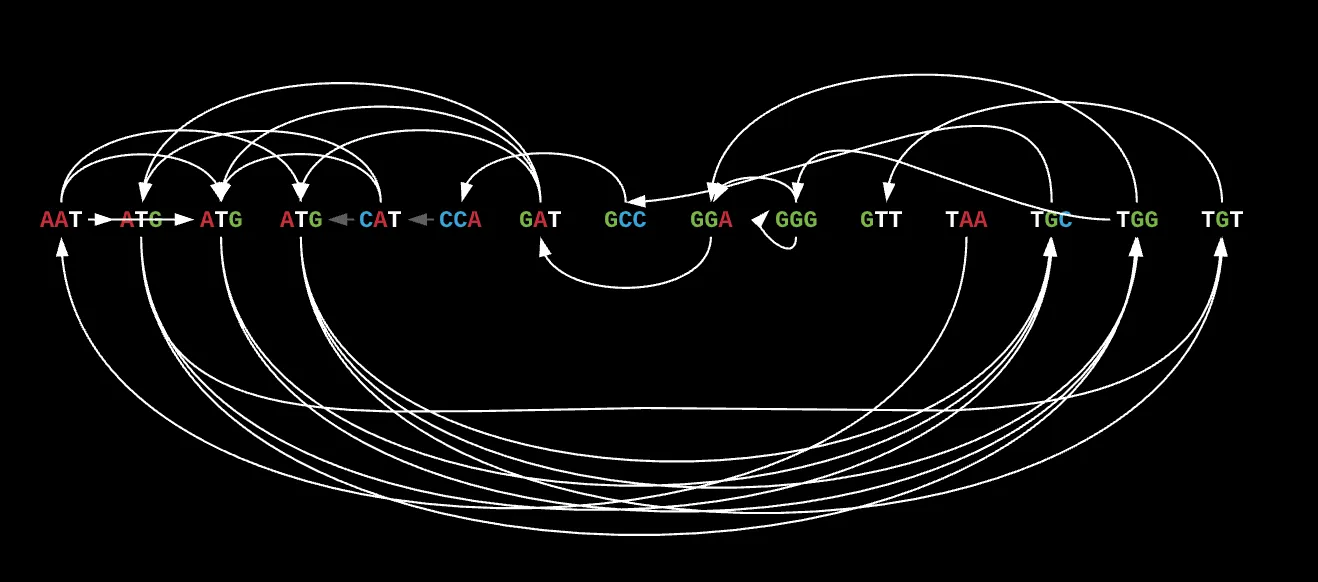
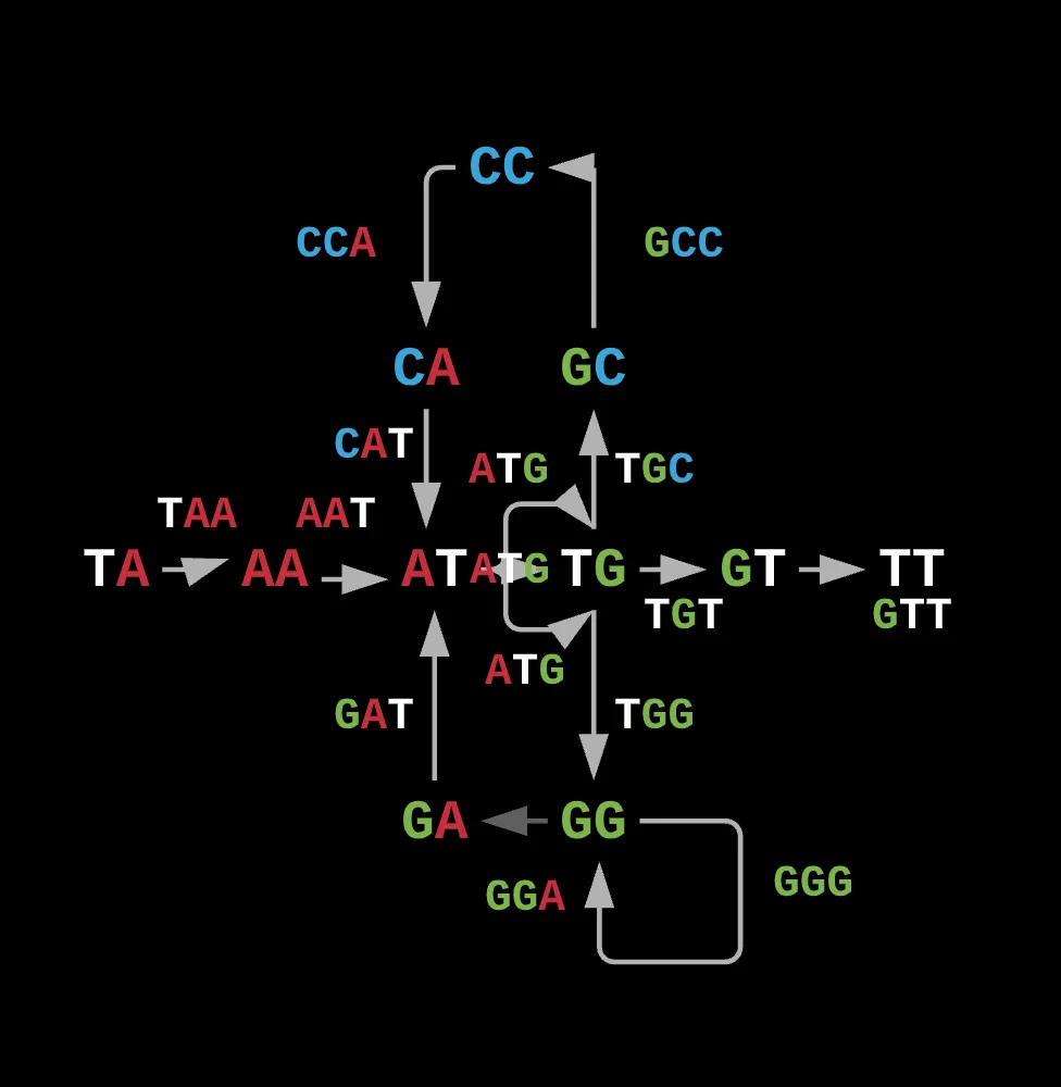
To highlight this, let’s take TAATGCCATGGGATGTT. If we look at its k-mer composition in lexicographic order, you would get

[‘AAT’, ‘ATG’, ‘ATG’, ‘ATG’, ‘CAT’, ‘CCA’, ‘GAT’, ‘GCC’, ‘GGA’, ‘GGG’, ‘GTT’, ‘TAA’, ‘TGC’, ‘TGG’, ‘TGT’].

Note this applies for any k-mer specified.

If you remember correctly from the brute force method we had initially that motivated the idea of paths for decision making, you’ll know that another possible reconstruction of the initial sequence could be TAATGGGATGCCATGTT.

If you look at this sequence’s k-mer composition, it also happens to be

[‘AAT’, ‘ATG’, ‘ATG’, ‘ATG’, ‘CAT’, ‘CCA’, ‘GAT’, ‘GCC’, ‘GGA’, ‘GGG’, ‘GTT’, ‘TAA’, ‘TGC’, ‘TGG’, ‘TGT’]

This is the same k-mer composition as the previous sequence’s while they are both significantly different. What this entails to is that some graphs can have MULTIPLE Eulerian paths, which complicates our entire process.

But, if we increased our k-length from just 3 to 5, you can easily see that this problem is avoided for that one 5-mer.

[‘AATGC’, ‘ATGCC’, ‘ATGGG’, ‘ATGTT’, ‘CATGG’, ‘CCATG’, ‘GATGT’, ‘GCCAT’, ‘GGATG’, ‘GGGAT’, ‘TAATG’, ‘TGCCA’, ‘TGGGA’]

[‘AATGG’, ‘ATGCC’, ‘ATGGG’, ‘ATGTT’, ‘CATGT’, ‘CCATG’, ‘GATGC’, ‘GCCAT’, ‘GGATG’, ‘GGGAT’, ‘TAATG’, ‘TGCCA’, ‘TGGGA’]

CATGG and CATGT do not match since with a longer read length, there is less room for repeats. Now, in the context of a 3 billion long genome and a maximum cap of 300-long nucleotides, this problem can become complicated really fast.

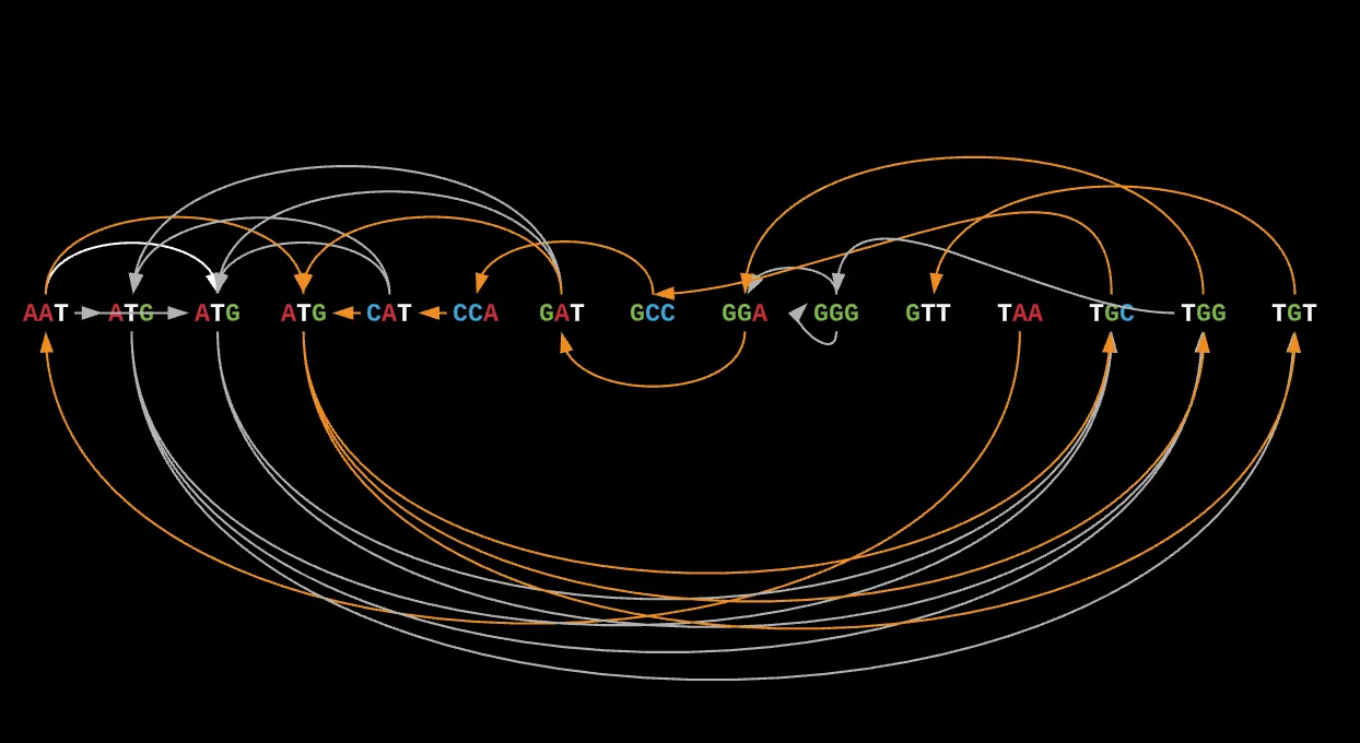
If I were to pass the De Bruijn representation for a contig set shown above, I would get 2 different Eulerian paths as solutions to the problem.

For just this one example, we could have easily considered that there was an error in our sequencing which caused just 1 nucleotide to be wrong. This is a completely fair assumption to make, yet the final outcome can diverge dramatically.

Thankfully, there is a way to solve this conundrum, and it comes with our initial sequencing process.

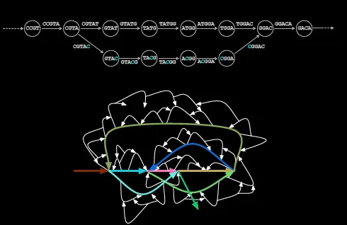
When we shotgun sequence our initial genome several times, you get longer, random areas of overlap that differ across several copies.

In our initial approach, we would have only been able to assemble a single sequence but never overlapping sequences. We want to get the magenta and teal overlap sequences with just their collective set of contigs. How can we do this given a series of k-mers that represent areas of overlap across sequences?

Let’s jump into something known as Paired Composition Graphs.

A paired composition graph is essentially several pairs of reads that are separated by a set distance.

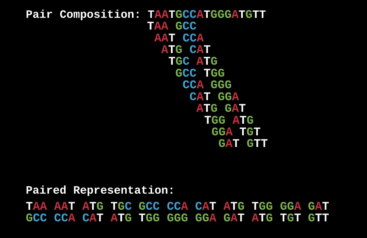
This is a (3, 1) paired read composition as every read has a distance of 1 nucleotide between it. What you’ve done with this representation is that you now have drawn connections between reads and gaps in such a way where the overlap of these pairs can only correspond to 1 specific sequence and nothing else.

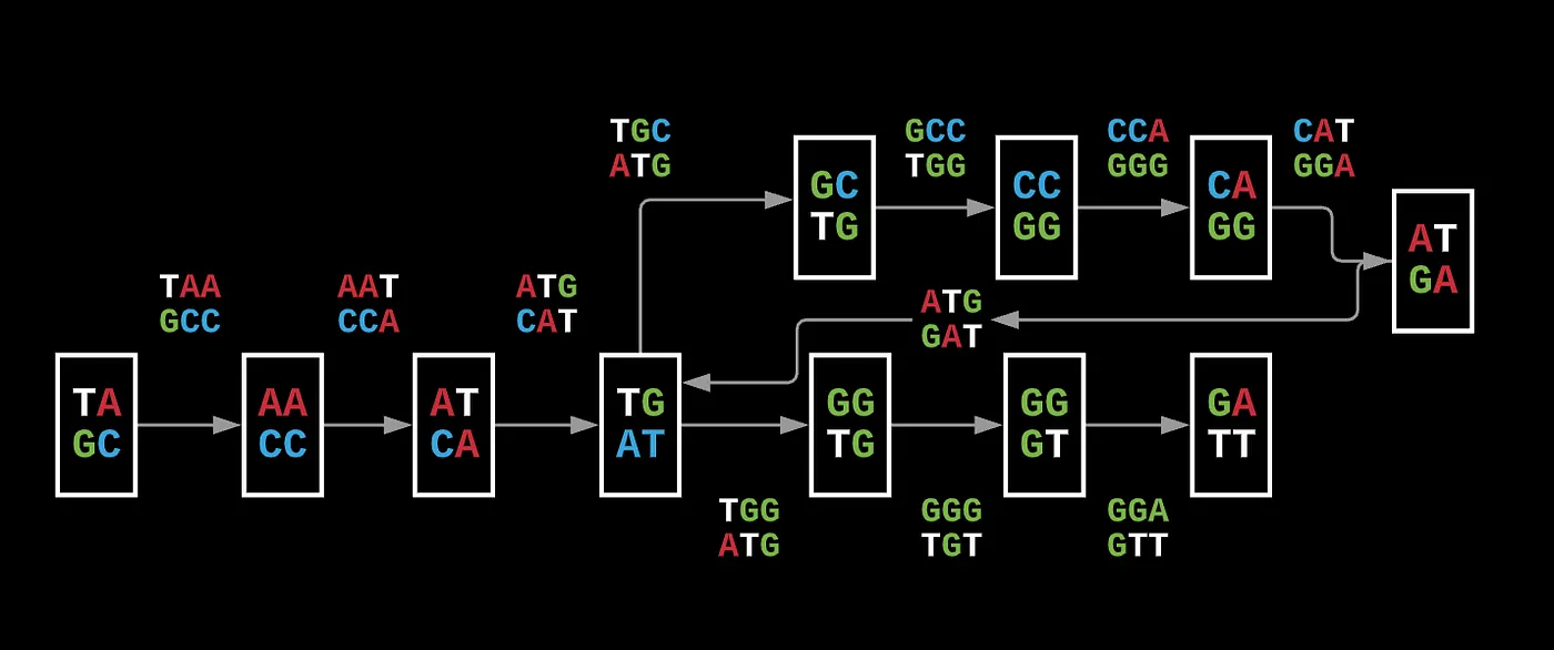
You can still represent this as a set of nodes and edges in a De Bruijn graph, but now each edge is a pair of reads and the nodes are the paired prefixes and suffixes of each read in the pair. To see why this representation is much more useful, we can look at the previous De Bruijn graph.

Let’s say we have CCA and AAT, in a pairwise representation, you have a unique string spelled by paths of length 5 (that’s ultimately the final overlap) but instead of having the additional sequence that’s redundant, you can write AAT-CCA which shows that there is a longer path of 2k + d.

If you did overlap it, you would get AATGCCA where now you’ve encoded AAT, ATG, TGC, GCC, and CCA in a 5-length mer instead of 3 * (k=3) mer.

This also eliminates unnecessary repeats and allows you to simplify your potential paths without having to substantially increase the length of your reads by eliminating the repetition for ATG.

Using this system, the goal is to use coverage to your advantage as since you can now have 2 specific paths with a large area of coverage, they would need to match up without any errors.

To illustrate this, we can look at the same example we had with identical k-mer sets and now use our pair-wise composition to compare the two TAATGCCATGGGATGTT and TAATGGGATGCCATGTT respectively.

[‘TAA|GCC’, ‘AAT|CCA’, ‘ATG|CAT’, ‘TGC|ATG’, ‘GCC|TGG’, ‘CCA|GGG’, ‘CAT|GGA’, ‘ATG|GAT’, ‘TGG|ATG’, ‘GGG|TGT’, ‘GGA|GTT’]

[‘TAA|GGG’, ‘AAT|GGA’, ‘ATG|GAT’, ‘TGG|ATG’, ‘GGG|TGC’, ‘GGA|GCC’, ‘GAT|CCA’, ‘ATG|CAT’, ‘TGC|ATG’, ‘GCC|TGT’, ‘CCA|GTT’]

The difference between the pairs is clear, and it helps differentiate between different paths while optimizing for a single solution.

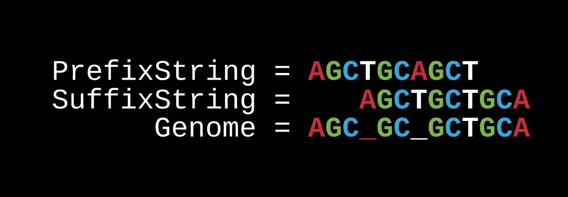
Another point about the pairs is that they are useful because they represent the prefix and suffix of the read we are focusing on.

In the case of the string AGCAGCTGCTGCA, it can be spelled by the path AG-AG → GC-GC → CA-CT → AG-TG → GC-GC → CT-CT → TG-TG → GC-GC → CT-CA.

Through the overlap, you would get AGCAGCTGCTGCA which matches.

But if we switched to another potential Eulerian path, the order of the paired-reads would be AG-AG → GC-GC → CT-CT → TG-TG → GC-GC → CA-CT → AG-TG → GC-GC → CT-CA.

The overlap however would not work as now you would get different nucleotides: AGC?GC?GCTGCA.

We can use a similar approach for formulating the De Bruijn graph of a given set of pair-reads where the nodes (prefix or suffix of both pairs) only connects to the other if the suffix of the current_node = the prefix of the next_node (thus showing overlap).

The following code can be used to convert a set of pair-reads into a De Bruijn.

And from there, we can use the exact same Eulerian Path algorithm from before.

To assemble the final genome, we use the approach demonstrated above where we can find the overlap area using the following function:

Given the following example:

4 2
GAGA|TTGA
TCGT|GATG
CGTG|ATGT
TGGT|TGAG
GTGA|TGTT
GTGG|GTGA
TGAG|GTTG
GGTC|GAGA
GTCG|AGAT

Your final reconstruction will be GTGGTCGTGAGATGTTGA where k=4, d=2.

Okay, now time to address some practical parts of genome assembly.

You’ve probably noticed that there are a lot of assumptions made here. For one, coverage was always assumed to be perfect for each genome which is often not true.

In fact, coverage is always imperfect. Illumina’s sequencing technology, regarded as the best in the world, is able to sequence 300-mer reads but misses several key contigs. And the ones that it does pick up tend to always have errors.

Despite this, the company has made several improvements outlined in their white paper here.

In order to really solve the coverage and accuracy problem, most modern assemblers use a read-breaking approach where they take several long contigs and break them up into read-pairs using an FM index. After, using the index of the contigs on the genome, you can cross-over the read-pairs to achieve perfect coverage.

As a result, you can use our current process to work with the ambiguity of assembling read-pairs but then use the indexed positions of the contigs across the genome to align the k-mers in the read-breaking approach with an O(logN) complexity.

Indexing contigs not only removes transitive edges in the graph, but also condenses our representation to untangle our graph. When we use this with our read-pairs to find gaps in the scaffold and fill them in.

At the same time, the size of reads is critical like we outlined before, where a smaller k-mer will increase the total coverage given enough DNA copies and areas of overlap but will also make our graph more computationally expensive.

We can often model De Bruijn graphs with other hyperparameters such as the minimum or maximum overlap length which can create several branches and paths for an ideal Eulerian path solution to the minimum hamming distance between the overlapping segment and the actual read.

Hamming distance and entropy are measures of variation between a set of sequences. A hamming distance of 0 means that all sequences in the set are identical, and anything higher signifies that there are multiple base pair differences.

Entropy can be considered as the probability distribution that models the mismatched variation between a set of sequences.

Topical entropy is typically useful for modelling weighted graphs where we can use lower entropy as a sign that there is a greater chance that the overlap between 2 or more reads are accurate.

[[0.2 0.2 0.  0.  0.  0.  0.9 0.1 0.1 0.1 0.3 0. ]  
 [0.1 0.6 0.  0.  0.  0.  0.  0.4 0.1 0.2 0.4 0.6]  
 [0.  0.  1.  1.  0.9 0.9 0.1 0.  0.  0.  0.  0. ]  
 [0.7 0.2 0.  0.  0.1 0.1 0.  0.5 0.8 0.7 0.3 0.4] ]

The first output is the count matrix which models the probability distribution of a nucleotide for a given position in the sequence. For example, the first column of the matrix has 0.7 for T signifying that the optimal overlap area would start with nucleotide T.

The entropy as a result is the sum of the entropy for each individual row, thus at 9.916290005356972.

You can use a similar approach to find portions of a genome that occur multiple times with mismatching bases. You can use entropy to calculate an optimal coverage using a conserved overlap, after which you can prune that mismatch in the node and remove bubbles (which we’ll get into a little later).

Typically, most genomes cannot be assembled from start to finish so this is a critical step not only because it is expensive or modern tech cannot sequence longer strands, but sequencing an entire genome at the same time is prone to several errors, especially for De Novo.

Most sequencing applications are based on Whole Genome Sequencing where you construct the entire organism’s genome using assembly, and this approach is accurate because there is reference material for most organisms through years of study.

For De Novo approaches in relation to entirely foreign organisms, it becomes more difficult. The read-break approach however allows for the individual to analyze key variants with scope as most reads typically have ulterior functions.

These can be transcription factor binding sites, origin sites for replication, transposable elements, ribosomal rRNA genes, and satellite DNA. Base information helps identify mutations and maps function through assembly and better improves the process each time.

The multiplicity of our genome can often bring issues in assembly, but it also helps in creating accurate reference material which plays a big role in each and every major part in the health system from clinical care, diagnosis of rare diseases, and formulating personalized therapeutics and treatments.

Regardless, if there were to be a single nucleotide error that could not be accounted for, our initial De Bruijn graph would have a missing edge, making it impossible to find a Eulerian path.

A good way to think about the contigs with respect to our genome is by looking at non-branching graphs in the De Bruijn graph.

If you can recount from our Eulerian cycle section, this is just the first random walk you would make where the nodes in this graph all have in(v) and out(v) of 1 for each intermediate node apart from the starting and ending as they both won’t have an in() or out() respectively.

In the case of contigs for our graph, you can think of this as the path that ends once a node has more than one edge or choice, thus this helps produce several non-branching paths.

What we’re looking for are MAXIMAL non-branching graphs which differ from non-branching paths as they could go through any set of nodes and closely resembles an initial random walk.

A maximal non-branching graph is really just any path that ends once there is more than one possible path (degree > 1) to take.

TAATGCCATGGGATGTT, has nine maximal non-branching paths that spell out the contigs TAAT, TGTT, TGCCAT, ATG, ATG, ATG, TGG, GGG, and GGAT → because of repeats, it becomes harder to infer a unique Eulerian path without using read pairs as they only work with perfect coverage and it’s often rare to get said read-pairs.

Error-prone reads where single points or nucleotides are changed are a major barrier for sequencing. Multiple errors of multiple length can produce several deviations from the original path.

This is known as a bubble which is defined by diverging and then converging paths of potential read arrangements.

In the case of human genome sequencing, you can identify most bubbles through a baseline genome and identify potential errors in the DNA sequence, but what if your goal is to catch said mutations?

De Bruijn graphs modelling entire genomes typically have millions of bubbles that have different kinds of errors which can create a very misleading picture. Inexact repeats, for example, plagued the Human Genome Project as a single point mutation in 1 repeat compared to the other would produce identical bubbles that make it more difficult to choose the correct repeat.

In most cases however, you can prune off the bubbles because they have low coverage but there is nothing concrete about removing errors that is streamlined across most assemblers.

Using all of these strategies, most industrial String Graph Assemblers often get 94%+ coverage on average and close to 99% for humans which is really great for getting an accurate picture of a patient.

Genome assembly can be considered the first foundational step for understanding the language that makes up all life.

A presumably simple part of the pipeline, assembly is a vital component of advancing the field of bioinformatics and computational biology.

To comment more on the practical use cases of assemblers, most services are based on mapping assemblers which utilizes reference-guided reconstruction of a known genome. Some open-sourced ones include AMOS (A Modular Open-Source Assembler**)** which includes tools for De Novo assembly and different tools such as generating scaffolds and overlap-graphs and, Illumina’s SPAdes for small genomes, and IDBA-UD, which although older, is open source.

It’s important to recognize that the role of computation has dramatically sped up our ability to assemble entire genomes on just 4GB of ram. Early technology built on termination and pyrosequencing has continued to help improve read-length with time and cost.

From sequencing to assembly, we’re essentially deciphering the genetic puzzle with clues and traits. Through this process, we’ve learned more than ever about several organisms and ourselves, and have been able to exploit the unique properties of certain genes based on their location and mode of expression to solve some fundamental problems.

We’re at a point now where sequencing technology seems to be the biggest barrier in improving computational methods for assembly, yet through some of the processes I’ve outlined in this article, bioinformaticians have been able to pioneer new fields and methods from comparative genomics to personalized medicine.

De novo assembly is still an important issue in the field, as Liao et al. states,

The first challenge is the sequencing errors, which possibly introduce artifacts in the assembly results… sequencing bias in platforms like Illumina’s have base composition bias which usually results in uneven sequencing depth. The third is the topological complexity of repetitive genomes (repeats account for 25–50% of entire mammalian genomes)… The last challenge is the huge computational resource consumption. Although the de novo assembly of small genomes, such as bacterial genomes, take only several minutes, the assembly of large genomes, such as mammalian genomes, typically takes several days to weeks and requires over tens to hundreds of GB of peak RAM memory

A lot of what I’ve learned through this process has better prepared me to not only take into account the practical barriers with genomics as a field while understanding a lot of the industry’s key problems, but I’m also excited to learn more and work on some of the more problematic aspects of assembly and analysis.

And I hope you now share the same enthusiasm towards the field of biology and engineering as I do.

More builds coming soon.

Thanks for taking the time to read this and I hope you got something out of it. If you want to get more technical or simply reach out to me, you can find me on_ LinkedIn, Email, or GitHub. Also Website [in works because nothing works :)]. You can also subscribe to my newsletter here.

I’m going to be on this CS/DL/CB train for a much longer time now, so if you have any cool papers, ideas, tech, or people I should know about/talk to, I would really appreciate that.

Some of the resources I consulted that you should check out (esp. 5, 1, and 8).

1. https://www.bioinformaticsalgorithms.org/ 2. https://link.springer.com/content/pdf/10.1007/s40484-019-0166-9.pdf 3. https://www.ncbi.nlm.nih.gov/pmc/articles/PMC3072823/ 4. http://www.cs.toronto.edu/~ashe/ham-path-notes.pdf 5. https://www.youtube.com/watch?v=xR4sGgwtR2I 6. https://www.youtube.com/watch?v=otOipgZF0ag 7. https://www.youtube.com/watch?v=5wvGapmA5zM 8. https://www.youtube.com/watch?v=ZYW2AeDE6wU 9. https://www.youtube.com/watch?v=KASvlXYPCBI